Chapter 2 Cluster analysis

2.1 Data preparation

For the purpose of demonstration we will be using a subsample from the larger data set.

set.seed(133)
n = 200
val_sub <- data_val %>%
  drop_na() %>% 
  group_by(country) %>% 
  sample_n(n) %>% 
  ungroup() %>% 
  dplyr::select(-country)

#libraries for this chapter
library(cluster)    # clustering algorithms
library(factoextra) # clustering algorithms & visualization

The data pre-processing involves two main steps: - remove variables with near zero variance - scale the data (Z-scores with mean as the center, and sd for spread); one could potentially make an argument for using mean average deviation for estimating the spread of the data.

val_sub <- val_sub[,-caret::nearZeroVar(val_sub)] #remove columns with near zero variance - we have already removed the columns with near zero variance so we move to the next step. 
val_sub<- val_sub %>% 
  scale()

#Let's take a look at the data 
df <- val_sub %>% 
  data.frame() 
df %>% 
   mutate_if(is.numeric, ~round(., 2)) %>% 
   reactable()

2.2 K-means Clustering

This type of Clustering involves minimizing the within cluster variation. Hartigan and Wong(1979) provided the following algorithm for K-means Clustering

\[W(C_k) = \sum_{x_1 \in C_k}(x_i-μ_k)^2\] where \(x_i\) is a data point in cluster \(C_k\) and \(μ_k\) is the mean of all values in cluster \(C_k\).To put it simply, Clustering is an optimization algorithm which and k-means is one variant which tries to build coherent clusters that minimize within cluster dissimilarity.

2.2.1 How to specify the number of clusters?

One of the important questions across dimension reduction techniques involves how many dimensions are the most optimal to describe the data at hand. This is essentially what we intend to do when we want to identify the groups in the data given the features. In our case the features involve the use variables in the World Value Survey.

Method WSS: The within cluster dispersion of data, also know as the error measure, is likely to drop more prominently after some clustering value. This creates a “elbow” like visual on the plot which is utilized to indicate the optimal number of clusters to model the data.

fviz_nbclust(
  val_sub, 
  kmeans, 
  method = "wss", 
  k.max = 50, 
  nboot = 200
  ) + 
  theme_minimal() + 
  ggtitle("Method: WSS [Elbow method] ") + 
  geom_vline(xintercept = 5, linetype = 2)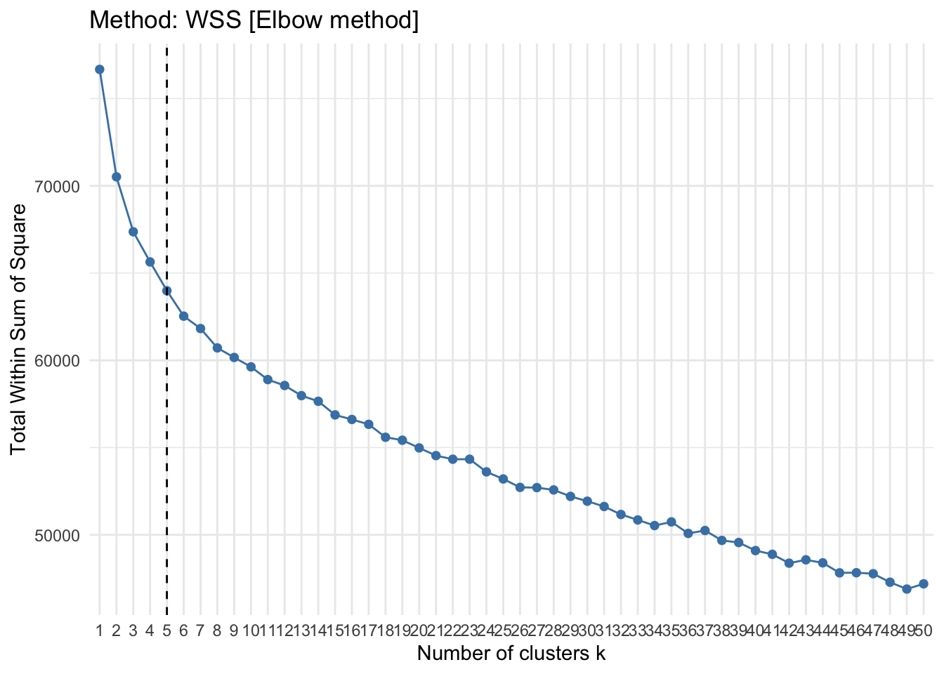

Method: Silhoutte: This method determines the appropriateness of a data point in a cluster. In other words, it computes how similar an observation is to a given cluster as compared to neighboring clusters. It computes average silhoutte of observations for varying k values. the k configuration is dependent on the values assigned to the observations across clusters, if these values are high the k or the number of clusters is seen as the appropriate value for structuring the data.

fviz_nbclust(
  val_sub,
  kmeans,
  method = "silhouette"
  ) + 
  theme_minimal() +
  ggtitle("Method: Silhouette")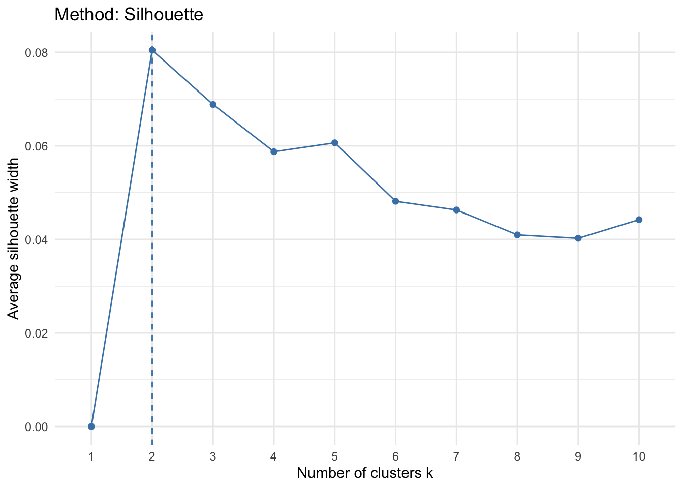

Method: Gap stat: This method computes pooled within cluster sum of squares and compares it to a null model of a single component.

fviz_nbclust(val_sub, kmeans, method = "gap_stat")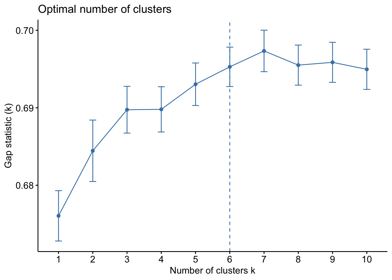

Sum of square : This method relies on minimizing the within cluster variance and increasing between cluster variance.

#Function to run this algorithm on 

pull_vals <-  function(n_center) {
  
  n_center <- {{n_center}}
  withinness <- mean(kmeans(val_sub, center = {{n_center}})$withinss)
  betweenness <-  kmeans(val_sub, center = {{n_center}})$betweenss
  
   l = list(n_center, withinness, betweenness) 
   names(l) <- c("n_center", "withinness", "betweenness")
   l
}

ssc <- map_df(1:40, pull_vals)

plot_ssc <- ssc %>%
  gather(key = "measurement", value = value, -n_center)

plot_ssc %>% 
    ggplot(aes(x = n_center, y = log10(value), fill = measurement)) +
       geom_bar(stat = "identity", position = "dodge", alpha = .8) +     
       labs(x = "Number of Clusters", 
            y = "Log10 Total Sum of Squares", 
            title = "Cluster Model Comparison") +
       scale_x_discrete(name = "Number of Clusters", limits = paste0(1:40)) +
       geom_hline(aes(yintercept = 4.5), linetype = 3, size = .2, alpha = .5)+
       theme_minimal()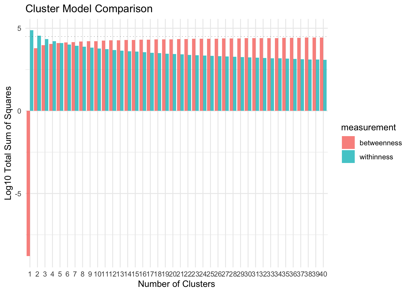

As you can see in the plot above, the WSS drop as the number of clusters increase. It keeps dropping even when the cluster size is 40. The graph indicates that the between cluster variance does not increase by much after k = 35. We can consider this as an approximate of the value of optimal k for the data.

Method: Bayesian Inference Criterion [BIC]

library(mclust)
d_clust <- Mclust(as.matrix(val_sub), G=1:15, 
                  modelNames = mclust.options("emModelNames"))

plot(d_clust)

Method: Average of 30 indices The NbClust package in R contains up to 30 indices (for example, Hartigan (1975),Ratowsky and Lance(1978), etc. ) for determining the number of appropriate clusters.

#Check with Talapas 
library(NbClust)
# res.nbclust <- NbClust(val_sub, distance = "euclidean", min.nc = 2, max.nc = 9, method = "complete", index ="all")
# 
# factoextra::fviz_nbclust(res.nbclust) + 
#    ggtitle("NbClust's optimal number of clusters") + theme_minimal()

res.nbclust_15 <- NbClust(
  data,
  distance = "euclidean",
  min.nc = 2,
  max.nc = 15,
  method = "complete",
  index ="all"
)

# the rest of this chunk should be cleaned up too

factoextra::fviz_nbclust(res.nbclust)

res.nbclust_15 <- NbClust(val_sub, distance = "euclidean", min.nc = 2, max.nc = 15,method = "complete", index ="all")

factoextra::fviz_nbclust(res.nbclust_15) + 

   ggtitle("NbClust's optimal number of clusters") + theme_minimal()

res.nbclust_15$Best.nc %>% as_tibble() %>% pivot_longer(cols = KL:SDbw,  names_to = "index") %>% slice(1:26) %>% count(value) %>% 
  ggplot(aes(x = factor(value), y = n))+
  geom_col(fill = "#F08080", alpha = .8)+
  theme_minimal() +
  labs(title = "NbClust's optimal number of clusters", 
       x = "Number of clusters k",
       y = "Frequency among all indices")

Hierarchical clustering We will set the distance method to euclidean. The linkage method we will be using here is the average linkage method. This algorithm will need a higher computing power given the large data and number of computations.

hc_data <- val_sub
dist_mat <- dist(val_sub, method = 'euclidean')
hclust_avg <- hclust(dist_mat, method = 'average')
#plot(hclust_avg) - aborts session, data is too big

Cluster tree This algorithm is helpful in considering various custering choices. The visual analysis of the clustering tree indicates how sample sizes in clusters change as the number of clusters increases. The node size corresponds to the sample size in a specific cluster. One way of looking at this method is to come up with candidate models for then identifying the most robust model.

library(clustree)
tmp <- rep(NA, 11)
for (k in seq_along(tmp)){
  tmp[k] <- kmeans(val_sub, k, nstart = 30)
}
df <- data.frame(tmp)
# add a prefix to the column names
colnames(df) <- seq(1:11)
colnames(df) <- paste0("k",colnames(df))
# get individual PCA
df.pca <- prcomp(df, center = TRUE, scale. = FALSE)
ind.coord <- df.pca$x
ind.coord <- ind.coord[,1:2]
df <- bind_cols(as.data.frame(df), as.data.frame(ind.coord))
clustree(df, prefix = "k")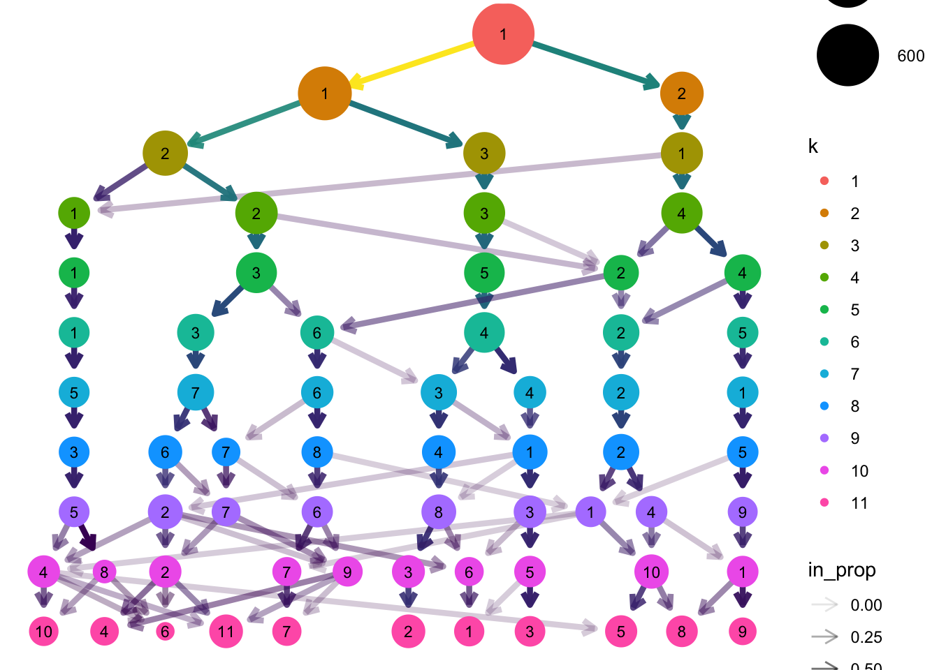

# The below needs styled
df_subset <- df %>% select(1:8,12:13)
clustree_overlay(df_subset, prefix = "k", x_value = "PC1", y_value = "PC2")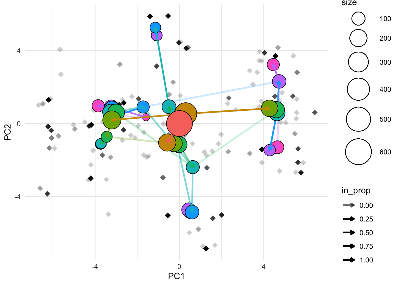

overlay_list <- clustree_overlay(df_subset, prefix = "k", x_value = "PC1",
                                 y_value = "PC2", plot_sides = TRUE)
overlay_list$x_side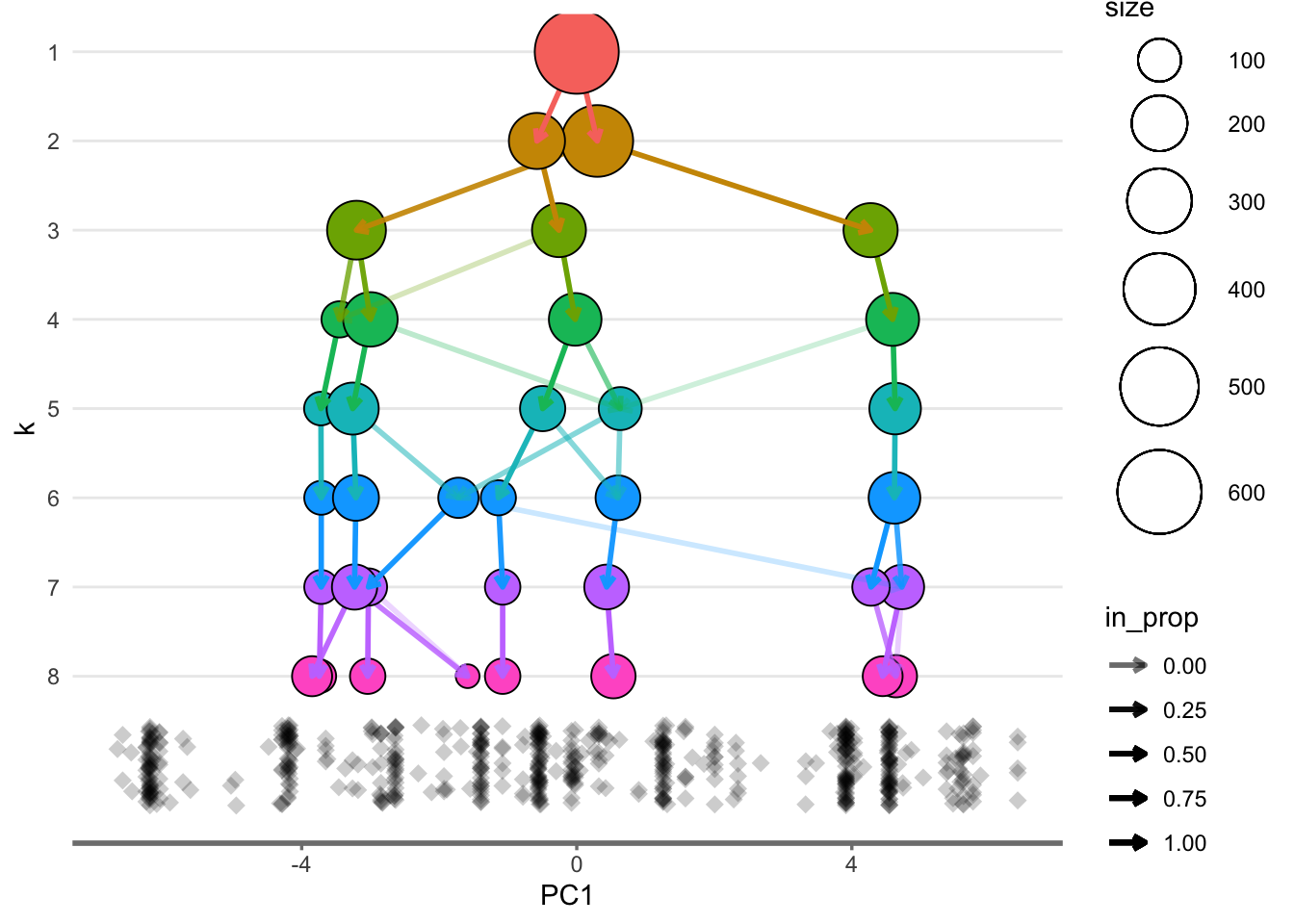

overlay_list$y_side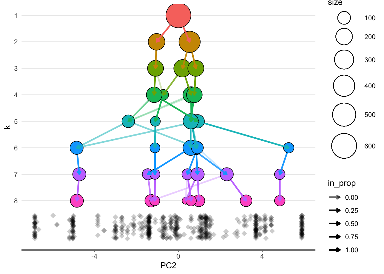

2.3 Conclusion

Cluster analysis is going to be an important consideration for determining the most optimal number of clusters for the given research question. I am particularly inclined to use divisive hierarchical clustering or a related variant of the same.