Chapter 3 Network Analysis

One way of conceptualizing meaningful cultural groupings could involve using the idea of networks consisting of nodes and edges. A common way of representing graphs in social network analysis involves representing nodes as people where th edges indicate some mathematical relation between the nodes. As a thought experiment one could think of these edges as psychological distances between people. The valence (positive or negative) of these edges could indicate similarity (or dissimilarity) in the thought processes of people. The weights of these edges (indicated by the thickness of the edges in the graph) could indicate the magnitude or strength of the similarity (or dissimilarity) in the thought processes of people. Once we are able to conceptualize the edges as thinking patterns, we need a way to find meaningful clusters or communities in the graph that will indicate groups that are similar to each other in their ways of thinking. Identification of such groups will involve algorithms that seek to find commonalities in the nodes and group them according to other similar nodes. This process in network analysis can be defined as community detection.

3.1 Community detection

The conceptual understanding of communities in the real world involves a level of consensus or agreement between members of the same community. For the purpose of demonstration we will be modeling psychological distances as personality variables and as Emancipative values. The community detection algorithms allow for mathematically modeling this idea of identifying clusters or communities in a network of participants which could be potential proxies of culture relevant groups in the data.

#Libraries
library(igraph)
library(psych)

3.2 Personality data

set.seed(229)
#222 gave a sd = 0

library(psych)
#Raw data 
data_bfi <- bfi %>% 
  dplyr::select(-gender, -education, -age) %>% 
  drop_na() %>% 
  sample_n(200) %>% 
  # rowwise() %>% 
  # mutate(A = sum(c(A1, A2, A3, A4,A5)),
  #        C = sum(c(C1, C2, C3, C4,C5)),
  #        N = sum(c(N1, N2, N3, N4, N5)),
  #        O = sum(c(O1, O2, O3, O4, O5)),
  #        E = sum(c(E1, E2, E3, E4, E5))) %>% 
  # dplyr::select(A, C, N, O, E) %>% 
  t() %>% 
  as.data.frame() %>% 
  janitor::clean_names() %>% 
  rename_all(funs(stringr::str_replace_all(., 'v', 'p'))) %>%
  cor()

#Ipsatized data
data_bfi_ip <- bfi %>% 
  select(-gender, -education, -age) %>% 
  drop_na() %>% 
  multicon::ipsatize() %>% 
  sample_n(200) %>% 
  t() %>% 
  as.data.frame() %>% 
  janitor::clean_names() %>% 
  rename_all(funs(stringr::str_replace_all(., 'v', 'p'))) %>%
  cor()

#Plot the correlations - raw
reshape2::melt(data_bfi) %>% 
  ggplot(aes(x=value)) +
     geom_density(fill="#69b3a2", color="#e9ecef", alpha=0.8)+
     labs(title = "Distribution of correlations - Raw data",
          x = "Range of correlation values")+
    theme_ipsum() +
    theme(plot.title = element_text(size=9))

#Plot the correlations - ipsatized
reshape2::melt(data_bfi_ip) %>% 
  ggplot(aes(x=value)) +
     geom_density(fill="#69b3a2", color="#e9ecef", alpha=0.8)+
     labs(title = "Distribution of correlations - Ipsatized data",
          x = "Range of correlation values")+
    theme_ipsum() +
    theme(plot.title = element_text(size=9))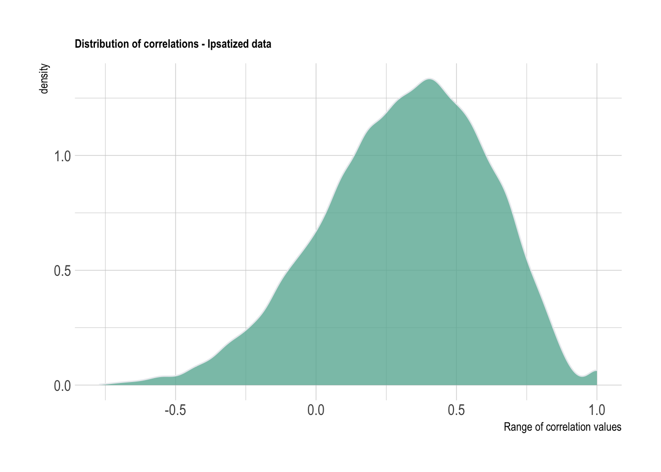

3.3 What is Community detection?

Community detection is the process of identifying similar nodes in a network. In order to find these similar nodes or communities we will be employing different algorithms based on Exploratory Graph analysis (EGA). EGA is a network psychometrics framework that intends to find clusters or communities within network models. The first step is to apply the graphical least absolute shrinkage and selector operator (GLASSO) to an inverse covariance matrix. This results in a Gaussian graphical model (or a network) wherein the edges are partial correlations and the nodes are targets. These targets are variables/features when applied to latent variable modeling. These targets would be, in our case, people. The networks would thus involve understanding the communities of participants in the data holding all the other connections constant (since we use partial correlation graphs). After estimating this graph we can further apply community detection algorithms to find the right connections between participants. The underlying framework for every community detection (CD) algorithm is slightly different from each other. We will be exploring the CD algorithms in the igraph package in R. Before we move on the algorithms it is important to understand one concept that will potentially affect the generation of these communities. The concept of modularity(Newman, 2006) is crucial to understanding any CD algorthim. Modularity in effect is the degree to which communities in a network have larger number of connections within the community in contrast to lesser connections outside the community.

$Q = 1 / 2 w Σ_{i j} (w_{i j} - \frac{w_{i} w_{j}}{2 w}) δ (c_{i}, c_{j})$ $w_{i j}$ = edge strength (e.g., correlation) between nodes $i$ and $j$ $w_{i}$ and $w_{j}$ = node strength (e.g., correlation) for nodes $i$ and $j$ $w$ = summation of all edge weights in the network $c_{i}$ , $c_{j}$ = community that node $i$ and node $j$ belong to $δ$ takes values 1 (when nodes $i$ and $j$ belong to the same community) and 0 (when nodes $i$ and $j$ belong to different communities) is 1 if the nodes belong to the same community (i.e., $c_{i} = c_{j}$ ) and 0 if otherwise.

Edge Betweenness This algorithm is based on the measure of betweenness cetrality in network graphs. The edge betweenness scores are computed based on how many shortest paths pass through a given edge in the network. The edge betweenness CD algorithm relies on the fact that edges with high betweenness are likely to connect multiple groups as these will the only ways for different groups/communities in the network to stay connected. The edge with the highest betweenness value is removed, followed by recomputing of betweenness for the remaining edges. The new highest betweenness value is identified and removed followed by another round of recomputation. An optimal threshold is established using modularity.

# edge betweenness 
set.seed(98)
data_bfi_eb <- bfi %>% 
  select(-gender, -education, -age) %>% 
  drop_na() %>% 
  sample_n(70) %>% 
  t() %>% 
  as.data.frame() %>% 
  janitor::clean_names() %>% 
  rename_all(funs(stringr::str_replace_all(., 'v', 'p'))) %>% 
  cor()

# the below could be styled better, note the following line is > 80 chars
g <- graph.adjacency(data_bfi_eb , mode = "upper", weighted = TRUE, diag = FALSE)
e <- get.edgelist(g)
df <- as.data.frame(cbind(e,E(g)$weight))
df <-  graph_from_data_frame(df, directed = F)

eb <- edge.betweenness.community(df)
plot(eb, df)

Fast and Greedy This algorithm begins with considering every node as one community and uses heirarchical clustering to build communities. Each node is placed in a community in a way that maximizes modularity. The communities are collapsed into different groups once the modularity threshold has been reached (i.e. no significant improvement in modularity is observed). Due to the high speed of this algorithm it is often a preferred approach for quick approximations of communities in the data.

g <- graph.adjacency(data_bfi, mode = "upper", weighted = TRUE, diag = FALSE)
e <- get.edgelist(g)
df <- as.data.frame(cbind(e,E(g)$weight))
df <-  graph_from_data_frame(df, directed = F)

#Fast and greedy algorithm 
fg <- fastgreedy.community(df)
fg

## IGRAPH clustering fast greedy, groups: 2, mod: 5.8e-17
## + groups:
##   $`1`
##     [1] "p1"   "p2"   "p3"   "p4"   "p5"   "p6"   "p7"   "p8"   "p9"   "p10" 
##    [11] "p11"  "p12"  "p13"  "p14"  "p15"  "p16"  "p17"  "p18"  "p19"  "p20" 
##    [21] "p21"  "p22"  "p23"  "p24"  "p25"  "p26"  "p27"  "p28"  "p29"  "p30" 
##    [31] "p31"  "p32"  "p33"  "p34"  "p35"  "p36"  "p37"  "p38"  "p39"  "p40" 
##    [41] "p41"  "p42"  "p43"  "p44"  "p45"  "p46"  "p47"  "p48"  "p49"  "p50" 
##    [51] "p51"  "p52"  "p53"  "p54"  "p55"  "p56"  "p57"  "p58"  "p59"  "p60" 
##    [61] "p61"  "p62"  "p63"  "p64"  "p65"  "p66"  "p67"  "p68"  "p69"  "p70" 
##    [71] "p71"  "p72"  "p73"  "p74"  "p75"  "p76"  "p77"  "p78"  "p79"  "p80" 
##    [81] "p81"  "p82"  "p83"  "p84"  "p85"  "p86"  "p87"  "p88"  "p89"  "p90" 
##   + ... omitted several groups/vertices

# membership(fg)
# communities(fg)

Louvian This is similar to the greedy algorithm described above. This algorithm also uses heirarchical clustering. It intends to identify heirarchical structures wherein it swaps nodes between communities to assess improvement in modularity. Once the modularity reaches a point where no improvement is observes, the communities are modeled as latent nodes and edge weights with other nodes within and outside the community are computed. This provides a heirarchical or a multi-level structure to the communities identified. The results of Lovian and Fast Greedy algorithms are therefore, likely to be similar.

# Louvain
lc <- cluster_louvain(df)
lc

## IGRAPH clustering multi level, groups: 1, mod: 0
## + groups:
##   $`1`
##     [1] "p1"   "p2"   "p3"   "p4"   "p5"   "p6"   "p7"   "p8"   "p9"   "p10" 
##    [11] "p11"  "p12"  "p13"  "p14"  "p15"  "p16"  "p17"  "p18"  "p19"  "p20" 
##    [21] "p21"  "p22"  "p23"  "p24"  "p25"  "p26"  "p27"  "p28"  "p29"  "p30" 
##    [31] "p31"  "p32"  "p33"  "p34"  "p35"  "p36"  "p37"  "p38"  "p39"  "p40" 
##    [41] "p41"  "p42"  "p43"  "p44"  "p45"  "p46"  "p47"  "p48"  "p49"  "p50" 
##    [51] "p51"  "p52"  "p53"  "p54"  "p55"  "p56"  "p57"  "p58"  "p59"  "p60" 
##    [61] "p61"  "p62"  "p63"  "p64"  "p65"  "p66"  "p67"  "p68"  "p69"  "p70" 
##    [71] "p71"  "p72"  "p73"  "p74"  "p75"  "p76"  "p77"  "p78"  "p79"  "p80" 
##    [81] "p81"  "p82"  "p83"  "p84"  "p85"  "p86"  "p87"  "p88"  "p89"  "p90" 
##   + ... omitted several groups/vertices

# membership(lc)
# communities(lc)
# plot(lc, g)

Walktrap This algorithm starts with computing a transition matrix $T_{i j}$ in which each matrix element $p_{i j}$ is the probability of one node $i$ traversing to another node $j$ .

$T_{i j} = [\begin{array}{rrr} p_{11} & p_{12} & p_{13} \\ p_{21} & p_{22} & p_{23} \\ p_{31} & p_{32} & p_{33} \end{array}]$

In the matrix above, $p_{32}$ is th probability that node 3 traverses to node 2 as determined by the node strengths of the two nodes. Ward’s agglomorative clustering approach is employed wherein nodes start off as a cluster of their own and then merge with adjacent clusters. The merging takes place in a way where the sum of squared distances between clusters are reduced.

#Random Walk 
wk <- walktrap.community(df)
wk

## IGRAPH clustering walktrap, groups: 200, mod: 0
## + groups:
##   $`1`
##   [1] "p1"
##   
##   $`2`
##   [1] "p2"
##   
##   $`3`
##   [1] "p3"
##   
##   $`4`
##   + ... omitted several groups/vertices

# membership(wk)
# communities(wk)

Infomap This is similar to the greedy walk algorithm except it converts the random walk information into a binary coding system. The partition of data into networks is carried out in a way that maximizes the information of random walks.

# Infomap
imc <- cluster_infomap(df)
imc

## IGRAPH clustering infomap, groups: 1, mod: 0
## + groups:
##   $`1`
##     [1] "p1"   "p2"   "p3"   "p4"   "p5"   "p6"   "p7"   "p8"   "p9"   "p10" 
##    [11] "p11"  "p12"  "p13"  "p14"  "p15"  "p16"  "p17"  "p18"  "p19"  "p20" 
##    [21] "p21"  "p22"  "p23"  "p24"  "p25"  "p26"  "p27"  "p28"  "p29"  "p30" 
##    [31] "p31"  "p32"  "p33"  "p34"  "p35"  "p36"  "p37"  "p38"  "p39"  "p40" 
##    [41] "p41"  "p42"  "p43"  "p44"  "p45"  "p46"  "p47"  "p48"  "p49"  "p50" 
##    [51] "p51"  "p52"  "p53"  "p54"  "p55"  "p56"  "p57"  "p58"  "p59"  "p60" 
##    [61] "p61"  "p62"  "p63"  "p64"  "p65"  "p66"  "p67"  "p68"  "p69"  "p70" 
##    [71] "p71"  "p72"  "p73"  "p74"  "p75"  "p76"  "p77"  "p78"  "p79"  "p80" 
##    [81] "p81"  "p82"  "p83"  "p84"  "p85"  "p86"  "p87"  "p88"  "p89"  "p90" 
##   + ... omitted several groups/vertices

# membership(imc)
#communities(imc)
# plot(fg, g)

Eigen vector This involves computing an eigenvector for the modularity matrix and splitting the network into communities in order to improve modularity. A stopping condition is specified to avoid tight communities to be formed. Due to eigenvector computations, this algorithm does not work well with degerate graphs.

# Eigen vector community
eg <- leading.eigenvector.community(df)
eg

## IGRAPH clustering leading eigenvector, groups: 1, mod: 0
## + groups:
##   $`1`
##     [1] "p1"   "p2"   "p3"   "p4"   "p5"   "p6"   "p7"   "p8"   "p9"   "p10" 
##    [11] "p11"  "p12"  "p13"  "p14"  "p15"  "p16"  "p17"  "p18"  "p19"  "p20" 
##    [21] "p21"  "p22"  "p23"  "p24"  "p25"  "p26"  "p27"  "p28"  "p29"  "p30" 
##    [31] "p31"  "p32"  "p33"  "p34"  "p35"  "p36"  "p37"  "p38"  "p39"  "p40" 
##    [41] "p41"  "p42"  "p43"  "p44"  "p45"  "p46"  "p47"  "p48"  "p49"  "p50" 
##    [51] "p51"  "p52"  "p53"  "p54"  "p55"  "p56"  "p57"  "p58"  "p59"  "p60" 
##    [61] "p61"  "p62"  "p63"  "p64"  "p65"  "p66"  "p67"  "p68"  "p69"  "p70" 
##    [71] "p71"  "p72"  "p73"  "p74"  "p75"  "p76"  "p77"  "p78"  "p79"  "p80" 
##    [81] "p81"  "p82"  "p83"  "p84"  "p85"  "p86"  "p87"  "p88"  "p89"  "p90" 
##   + ... omitted several groups/vertices

3.4 Values data

In this section we will apply all the previously learned algorithms to the Values data.

set.seed(133)
val_data <- data_val %>%
  group_by(country) %>% 
  sample_n(50) %>% 
  ungroup() %>% 
  dplyr::select(-country) %>%
  t() %>% 
  cor()

#Plot the correlations 
reshape2::melt(val_data) %>% 
  ggplot(aes(x=value)) +
     geom_density(fill="#69b3a2", color="#e9ecef", alpha=0.8)+
     labs(title = "Distribution of correlations - Values Raw data",
          x = "Range of correlation values")+
    theme_ipsum() +
    theme(plot.title = element_text(size=9))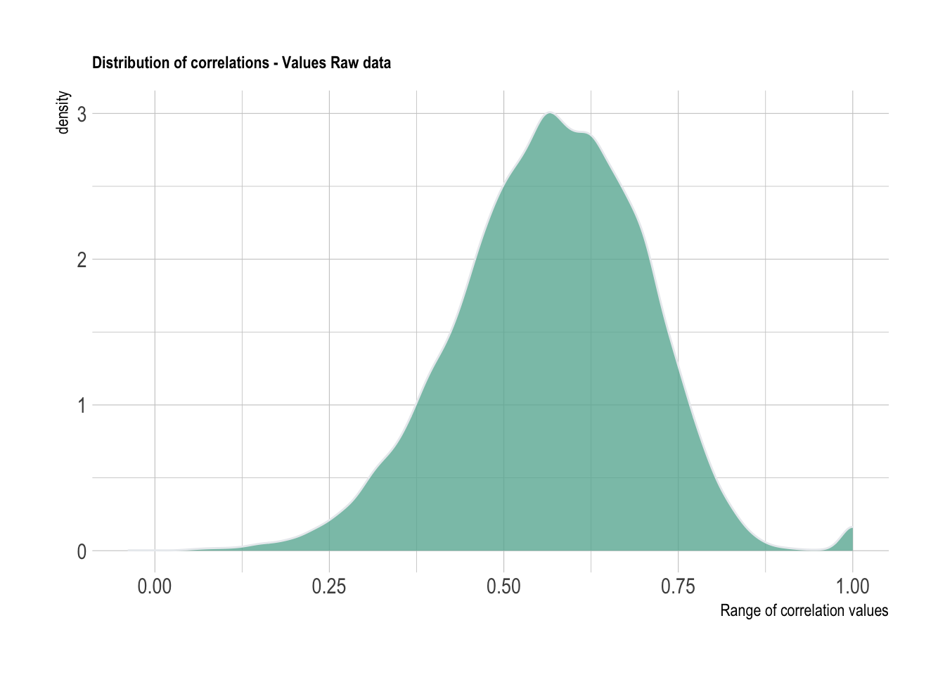

g <- graph.adjacency(val_data, mode="upper", weighted=TRUE, diag=FALSE)
e <- get.edgelist(g)
df <- as.data.frame(cbind(e, E(g)$weight))
df <- graph_from_data_frame(df, directed = FALSE)

# edge betweenness 
#eb <- edge.betweenness.community(df);eb
#plot(eb, df)

# Louvain
lc <- cluster_louvain(df)
lc

## IGRAPH clustering multi level, groups: 1, mod: 0
## + groups:
##   $`1`
##     [1] "1"   "2"   "3"   "4"   "5"   "6"   "7"   "8"   "9"   "10"  "11"  "12" 
##    [13] "13"  "14"  "15"  "16"  "17"  "18"  "19"  "20"  "21"  "22"  "23"  "24" 
##    [25] "25"  "26"  "27"  "28"  "29"  "30"  "31"  "32"  "33"  "34"  "35"  "36" 
##    [37] "37"  "38"  "39"  "40"  "41"  "42"  "43"  "44"  "45"  "46"  "47"  "48" 
##    [49] "49"  "50"  "51"  "52"  "53"  "54"  "55"  "56"  "57"  "58"  "59"  "60" 
##    [61] "61"  "62"  "63"  "64"  "65"  "66"  "67"  "68"  "69"  "70"  "71"  "72" 
##    [73] "73"  "74"  "75"  "76"  "77"  "78"  "79"  "80"  "81"  "82"  "83"  "84" 
##    [85] "85"  "86"  "87"  "88"  "89"  "90"  "91"  "92"  "93"  "94"  "95"  "96" 
##    [97] "97"  "98"  "99"  "100" "101" "102" "103" "104" "105" "106" "107" "108"
##   + ... omitted several groups/vertices

# membership(lc)
# communities(lc)
# plot(lc, g)

# Infomap
imc <- cluster_infomap(df)
imc

## IGRAPH clustering infomap, groups: 1, mod: 0
## + groups:
##   $`1`
##     [1] "1"   "2"   "3"   "4"   "5"   "6"   "7"   "8"   "9"   "10"  "11"  "12" 
##    [13] "13"  "14"  "15"  "16"  "17"  "18"  "19"  "20"  "21"  "22"  "23"  "24" 
##    [25] "25"  "26"  "27"  "28"  "29"  "30"  "31"  "32"  "33"  "34"  "35"  "36" 
##    [37] "37"  "38"  "39"  "40"  "41"  "42"  "43"  "44"  "45"  "46"  "47"  "48" 
##    [49] "49"  "50"  "51"  "52"  "53"  "54"  "55"  "56"  "57"  "58"  "59"  "60" 
##    [61] "61"  "62"  "63"  "64"  "65"  "66"  "67"  "68"  "69"  "70"  "71"  "72" 
##    [73] "73"  "74"  "75"  "76"  "77"  "78"  "79"  "80"  "81"  "82"  "83"  "84" 
##    [85] "85"  "86"  "87"  "88"  "89"  "90"  "91"  "92"  "93"  "94"  "95"  "96" 
##    [97] "97"  "98"  "99"  "100" "101" "102" "103" "104" "105" "106" "107" "108"
##   + ... omitted several groups/vertices

# membership(imc)
# communities(imc)
# plot(imc, g)

#Fast and greedy algorithm 
fg <- fastgreedy.community(df)
fg

## IGRAPH clustering fast greedy, groups: 2, mod: 1.9e-17
## + groups:
##   $`1`
##     [1] "1"   "2"   "3"   "4"   "5"   "6"   "7"   "8"   "9"   "10"  "11"  "12" 
##    [13] "13"  "14"  "15"  "16"  "17"  "18"  "19"  "20"  "21"  "22"  "23"  "24" 
##    [25] "25"  "26"  "27"  "28"  "29"  "30"  "31"  "32"  "33"  "34"  "35"  "36" 
##    [37] "37"  "38"  "39"  "40"  "41"  "42"  "43"  "44"  "45"  "46"  "47"  "48" 
##    [49] "49"  "50"  "51"  "52"  "53"  "54"  "55"  "56"  "57"  "58"  "59"  "60" 
##    [61] "61"  "62"  "63"  "64"  "65"  "66"  "67"  "68"  "69"  "70"  "71"  "72" 
##    [73] "73"  "74"  "75"  "76"  "77"  "78"  "79"  "80"  "81"  "82"  "83"  "84" 
##    [85] "85"  "86"  "87"  "88"  "89"  "90"  "91"  "92"  "93"  "94"  "95"  "96" 
##    [97] "97"  "98"  "99"  "100" "101" "102" "103" "104" "105" "106" "107" "108"
##   + ... omitted several groups/vertices

# membership(fg)
# communities(fg)

# Eigen vector community
eg <- leading.eigenvector.community(df)
eg

## IGRAPH clustering leading eigenvector, groups: 1, mod: 0
## + groups:
##   $`1`
##     [1] "1"   "2"   "3"   "4"   "5"   "6"   "7"   "8"   "9"   "10"  "11"  "12" 
##    [13] "13"  "14"  "15"  "16"  "17"  "18"  "19"  "20"  "21"  "22"  "23"  "24" 
##    [25] "25"  "26"  "27"  "28"  "29"  "30"  "31"  "32"  "33"  "34"  "35"  "36" 
##    [37] "37"  "38"  "39"  "40"  "41"  "42"  "43"  "44"  "45"  "46"  "47"  "48" 
##    [49] "49"  "50"  "51"  "52"  "53"  "54"  "55"  "56"  "57"  "58"  "59"  "60" 
##    [61] "61"  "62"  "63"  "64"  "65"  "66"  "67"  "68"  "69"  "70"  "71"  "72" 
##    [73] "73"  "74"  "75"  "76"  "77"  "78"  "79"  "80"  "81"  "82"  "83"  "84" 
##    [85] "85"  "86"  "87"  "88"  "89"  "90"  "91"  "92"  "93"  "94"  "95"  "96" 
##    [97] "97"  "98"  "99"  "100" "101" "102" "103" "104" "105" "106" "107" "108"
##   + ... omitted several groups/vertices

# communities(eg)

#Random Walk 
wk <- walktrap.community(df)
wk

## IGRAPH clustering walktrap, groups: 150, mod: 0
## + groups:
##   $`1`
##   [1] "1"
##   
##   $`2`
##   [1] "2"
##   
##   $`3`
##   [1] "3"
##   
##   $`4`
##   + ... omitted several groups/vertices

# membership(wk)
# communities(wk)

3.5 Conclusion

Community detection can effectively determine the number of groups in a data, however its important to remember that the centrality measures such as edge betweenness values are not comparable across simulations for a given number of nodes being considered. However, one could consider every node’s probablity of being in a specific group. The optimal number of group can be determined by considering the enitre dataset.