Chapter 4 Principal Component analysis

One of the most important algorithms used in dimensionality reduction is PCA. This method works very well with large datasets which makes it ideal for tasks such as this one.

4.1 Data Preparation

We will be working with a sample size of 50 from the Values data. This will be utilized for demonstrating the code. The problem of positive definite matrices although has not been completely solved at this point, the demonstrations are quite helpful.

# The below needs to be styled
# Note the inconsistent assignment operator
# lack of () on `t` and `cor`
# no line breaks after `%>%`
set.seed(133)
n = 50
data_PA <- data_val %>%
  drop_na() %>% 
  group_by(country) %>% sample_n(n) %>% ungroup %>% dplyr::select(-country) %>% 
  t %>% 
  cor

# alignment below needs work
data_PA %>% 
  reshape2::melt(value.name = "cor") %>% 
 ggplot(aes(x=cor)) +
     geom_density(fill="#69b3a2", color="#e9ecef", alpha=0.8)+
  labs(title = "Distribution of correlations - Values Raw data, n= 50",
       x = "Range of correlation values")+
    theme_ipsum() +
    theme(plot.title = element_text(size=9))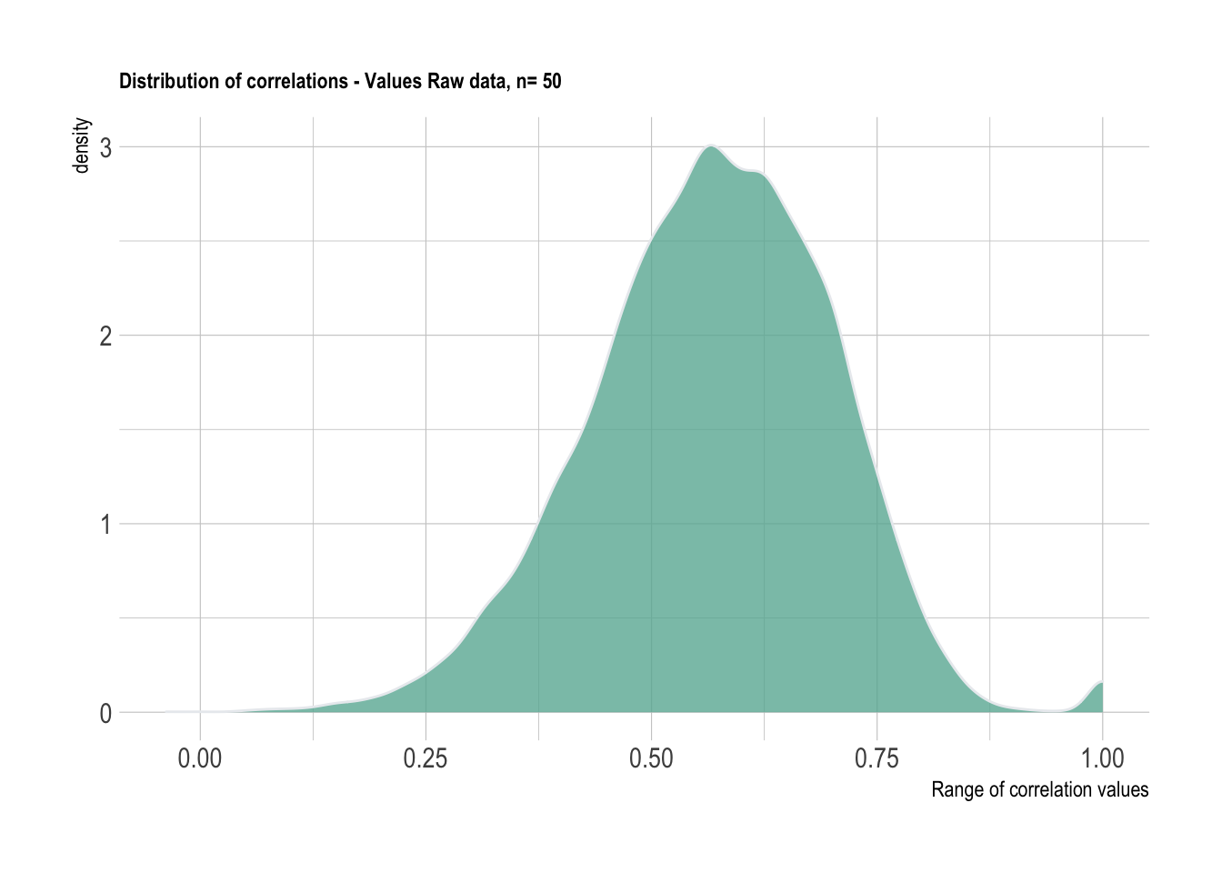

4.2 Parallel analysis (PA)

PA is considered to be one of the most trusted algorithms to determine the number of factors to be retained in a dataset. It has been proven to be more accurate than several other statistical methods such as the elbow method using the scree plot, Kaiser rule, or Velicer’s MAP test. Traditional PA compares eigenvalues (\(\lambda_1\)…\(\lambda_k\)) generated by the data at hand with averages of simulated eigenvalues (\(\bar{\lambda}_1\)…\(\bar{\lambda}_k\)). Correlation matrices consisting of the same dimensions are randomly generated a specific number of times and averages of all eigenvalues simulated are retained. The mean simulated eigenvalues are compared with the eigenvalues obtained in the data. When the \(\lambda_k\) > \(\bar{\lambda}_k\), you retain the eigenvalue. The number of eigenvalues retained is considered as the most optimum number for identifying the dimensionality of the data.

#Function for building Parallel analysis plots
PA_graph <- function(data){
  
  library(paran)
  library(scales)
  
  PA_allData <- paran({{data}}, iterations = 1000, centile = 0, quietly = TRUE, status = TRUE, all = TRUE, cfa = TRUE, graph = FALSE)

PA_df <- tibble(PA_allData$AdjEv,
                PA_allData$Ev,
                PA_allData$RndEv,
                PA_allData$Bias)

PA_df <- PA_df %>% 
  janitor::clean_names() %>% 
  tibble::rownames_to_column() %>% 
  mutate(rowname= as.numeric(rowname)) %>% 
  rename("pc" = rowname, 
         "adj_ev" = pa_all_data_adj_ev,
         "ev" = pa_all_data_ev, 
         "rnd_ev" = pa_all_data_rnd_ev,    
         "bias" = pa_all_data_bias) %>% 
  pivot_longer(cols = c(adj_ev, ev, bias)) 

PA_df %>% 
  ggplot(aes(x = pc, y = value, color = name))+
  geom_point(size = 1.5)+
  geom_line()+
  scale_x_continuous(name='Factor Number', breaks= pretty_breaks()) +
   scale_y_continuous(name='Eigenvalue', breaks= pretty_breaks()) +
  labs(legend_title = "Type of values")+
  scale_color_manual(values=c("#69b3a2", "#85C1E9", "#F5B041"))+
  geom_vline(xintercept = PA_allData$Retained, linetype = 'dashed', color = "#566573")+
  #geom_text(aes(x=10, label="Retain 5 components", y=40), position = position_dodge(width=0.9), colour="#566573", angle=90, size=2)+
  guides(color = guide_legend(title="Iteration type"))+
  theme_minimal() +
    theme(plot.title = element_text(size=9))
}

PA_graph(data_PA)

## 
## Using eigendecomposition of correlation matrix.
## Computing: 10%  20%  30%  40%  50%  60%  70%  80%  90%  100%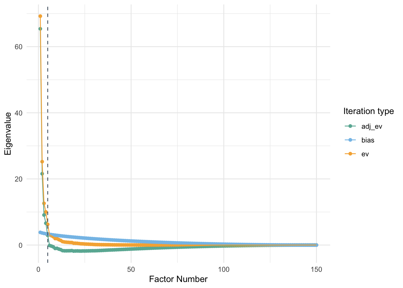

4.3 Personality data

One of the important things to recognize is that I need to remove rows that have zero variance. These participants have responded to the questionnaire with only one consistent option and this could cause issues with the correlation matrix estimation. This could also lead to issues is eigendecomposition of the matrix.

set.seed(900)
PA_pty <- bfi %>% 
  dplyr::select(-gender, -education, -age) %>% 
  drop_na() %>% 
  #slice(-drop_row) %>% 
  sample_n(200)  %>%  
  t %>%  
 cor()

PA_graph(PA_pty)

## 
## Using eigendecomposition of correlation matrix.
## Computing: 10%  20%  30%  40%  50%  60%  70%  80%  90%  100%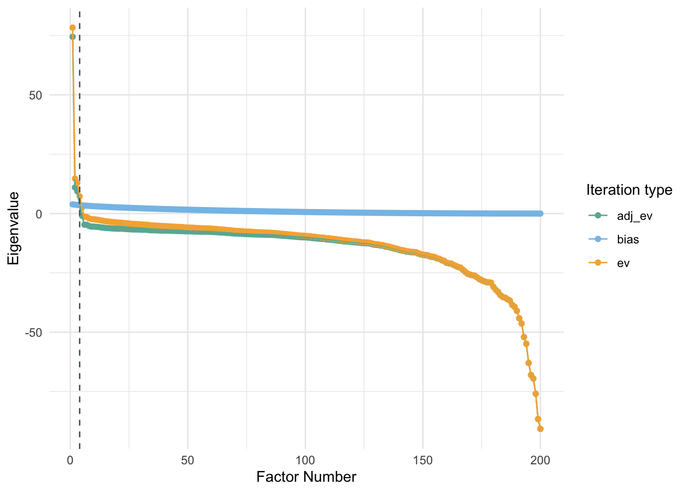

4.4 Bayesian Parallel Analysis

This is a relatively new method to compute Parallel analysis. We will be using a code from a recent paper to carry out this analysis.

One of the important considerations for this approach is understanding how this algorithm sets the initial number of dimensions to test. This approach requires a very high computation power. Following code can be used to apply this function to our data. The other thing to remember is that the matrices are often positive definite across multiple iterations and this problem needs to be addressed.

4.4.1 Personality data

library(matrixcalc)
#Personality data 
set.seed(18)
bfi %>% 
  dplyr::select(-gender,-education,-age) %>% 
  drop_na %>% 
  sample_n(20) %>% 
  t %>% 
  cor %>% 
   bayes.pa 

4.4.2 Values data

set.seed(453)
samp = 45
data_val %>% 
  group_by(country) %>%
  sample_n(samp) %>%
  ungroup %>%
    dplyr::select(-country, -V12, -V13, -V14, -V15, -V16, -V17, -V18, -V19, -V20, -V21, -V22) %>% 
  drop_na() %>% 
  mutate(id = paste0("p", 1:(samp*3))) %>% 
 ungroup %>% 
  t %>%
  data.frame %>% 
  janitor::clean_names() %>% 
  mutate_all(., as.integer) %>% 
  map_dfr(.,jitter) %>% 
  drop_na %>% 
  cor %>% 
  #is.positive.definite()
  bayes.pa 

4.5 Conclusion

I would like to explore more recent developments in parallel analysis wherein they have used a 95% confidence interval for every possible number of dimensions in the data. There needs to be a procedure for determining the most optimum number of dimensions for explaining the variance in the data. Perhaps I could set a specific amount of variance and a certain fraction of the total number of variables are criterion. More exploration is needed.